2-Node Corotational Beam (3D)
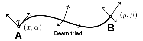
The beam consists of 2 nodes \(A\) and \(B\) at spatial coordinates \(\boldsymbol{x}, \boldsymbol{y} \in \mathbb{R}^3\).
Each node also has an assiciated triad (rotation of the standard basis),
parameterized by
\(\boldsymbol{\alpha}, \boldsymbol{\beta} \in \mathbb{R}^3\).
All nodal degrees of freedom are grouped together in the variable
\[
\boldsymbol{u} = (\boldsymbol{x}, \boldsymbol{\alpha}, \boldsymbol{y}, \boldsymbol{\beta}) \in \mathbb{R}^{12}.
\]
Moreover, the beam has the following properties:
- \(E\): Young's modulus,
- \(\nu\): Poisson's ratio,
- \(A\): beam area,
- \(I_y\): y area moment
- \(I_z\): z area moment
- \(J\)
The angular coordinates define a triad as follows:
For \(\boldsymbol{\theta} \in \mathbb{R}^3\), the corresponding
rotation is defined by
$$
R_{\boldsymbol{\theta}} := \exp([\boldsymbol{\theta}]_\times),
$$
where
\[
\begin{aligned}
\mathrm{exp}: \mathfrak{so}(3) & \rightarrow SO(3) \\
\mathrm{exp}(A) &= \mathbbm{1}
+ \frac{\sin(\|A\|)}{\|A\|} A + \frac{1-\cos(\|A\|)}{\|A\|^2} A^2, \qquad \|A\|^2 = -\frac{1}{2}\mathrm{tr}(A^2)
\end{aligned}
\]
is the matrix exponential series restricted to \(\mathfrak{so}(3)\) (skew symmetric matrices) and
\[
\left[ \boldsymbol{\theta} \right]_\times = \left(\begin{array}{rrr}
0 & -\theta_3 & \theta_2 \\
\theta_3 & 0 & -\theta_1 \\
-\theta_2 & \theta_1 & 0
\end{array}\right).
\]
A triad for given \(\boldsymbol{\theta} \in \mathbb{R}^3\) is then obtained as
the rotated Euclidean standard basis \(\boldsymbol{e}_1, \boldsymbol{e}_2, \boldsymbol{e}_3\):
\[
R_{\boldsymbol{\theta}} \boldsymbol{e}_1,
R_{\boldsymbol{\theta}} \boldsymbol{e}_2,
R_{\boldsymbol{\theta}} \boldsymbol{e}_3,
\]
i.e. the column vectors of \(R_{\boldsymbol{\theta}}\).
Note
In the simulation, the expressions for the energy, the force and the
stiffness will be evaluated at
\(\boldsymbol{u} = \boldsymbol{u}_0 + \delta \boldsymbol{u}\)
for some initial values \(\boldsymbol{u}_0\) and displacements
\(\delta \boldsymbol{u}\). As it does not make a difference to take the
derivative w.r.t \(\boldsymbol{u}\) or \(\delta \boldsymbol{u}\), we
will ommit \(\boldsymbol{u}_0\) and \(\delta \boldsymbol{u}\) and simply
use \(\boldsymbol{u}\) as the coordinates.
This is in contrast to [Crisfield], where
the angular coordinates \(\boldsymbol{\alpha}\) and \(\boldsymbol{\beta}\)
are not simply the sum of initial value plus displacement but are determined
by
\[
R_{\boldsymbol{\theta}} = R_{\boldsymbol{\theta}_0}R_{\delta\boldsymbol{\theta}},\qquad \theta=\alpha, \beta.
\]
We adapt the notation of [Crisfield] and denote
\[
\begin{aligned}
\boldsymbol{t}_i &= R_{\boldsymbol{\alpha}} \boldsymbol{e}_i,\quad i=1,2,3 \\
\boldsymbol{q}_i &= R_{\boldsymbol{\beta}} \boldsymbol{e}_i,\quad i=1,2,3.
\end{aligned}
\]
The average triad is obtained by applying the spherical linear interpolation:
\[
\label{eq:avg_triad}
\boldsymbol{r}_i = \mathrm{avg}(R_{\boldsymbol{\alpha}}, R_{\boldsymbol{\beta}}) \boldsymbol{e}_i,
\]
where
$$
\label{eq:avg}
\mathrm{avg}(R_{\boldsymbol{\alpha}}, R_{\boldsymbol{\beta}}) = (R_{\boldsymbol{\beta}} R_{\boldsymbol{\alpha}}^T)^{1/2} R_{\boldsymbol{\alpha}}
= (R_{\boldsymbol{\alpha}} R_{\boldsymbol{\beta}}^T)^{1/2} R_{\boldsymbol{\beta}}.
$$
For the beam triad, we differ from [Crisfield] as we already use \(\boldsymbol{e}_i\) for the standard basis and choose \(\boldsymbol{h}_i\) instead:
\[
\begin{aligned}
\boldsymbol{h}_1 &= \frac{\boldsymbol{y}-\boldsymbol{x}}{\|\boldsymbol{y}-\boldsymbol{x}\|},\\
\boldsymbol{h}_i &= \boldsymbol{r}_i - \langle \boldsymbol{r}_i, \boldsymbol{h}_1\rangle (\boldsymbol{h}_i + \boldsymbol{r}_1),\qquad i=2,3.
\end{aligned}
\]
Energy
The energy of the beam according to [Crisfield] is given by
\[
E = L_0 A e\left(\tfrac{\|\boldsymbol{y}-\boldsymbol{x}\|-L_0}{L_0}\right) + \frac{1}{2} \langle \boldsymbol{\ell}, D \boldsymbol{\ell} \rangle,
\]
where \(L_0\) is the initial value of \(\|\boldsymbol{y}-\boldsymbol{x}\|\),
\(e(\varepsilon)\) is the axial energy as a function of the axial strain,
\(\boldsymbol{\ell}\) is the vector of local rotational strains, defined by
\[
\begin{aligned}
2\sin(\boldsymbol{\ell}_1) &= -\langle \boldsymbol{t}_3, \boldsymbol{h}_2\rangle + \langle \boldsymbol{t}_2, \boldsymbol{h}_3\rangle,\\
2\sin(\boldsymbol{\ell}_2) &= -\langle \boldsymbol{t}_2, \boldsymbol{h}_1\rangle + \langle \boldsymbol{t}_1, \boldsymbol{h}_2\rangle,\\
2\sin(\boldsymbol{\ell}_3) &= -\langle \boldsymbol{t}_3, \boldsymbol{h}_1\rangle + \langle \boldsymbol{t}_1, \boldsymbol{h}_3\rangle,\\
2\sin(\boldsymbol{\ell}_4) &= -\langle \boldsymbol{q}_3, \boldsymbol{h}_2\rangle + \langle \boldsymbol{q}_2, \boldsymbol{h}_3\rangle,\\
2\sin(\boldsymbol{\ell}_5) &= -\langle \boldsymbol{q}_2, \boldsymbol{h}_1\rangle + \langle \boldsymbol{q}_1, \boldsymbol{h}_2\rangle,\\
2\sin(\boldsymbol{\ell}_6) &= -\langle \boldsymbol{q}_3, \boldsymbol{h}_1\rangle + \langle \boldsymbol{q}_1, \boldsymbol{h}_3\rangle,
\end{aligned}
\]
and
$$
D = \frac{1}{L_0} \left[
\begin{array}{cccccc}
GJ & 0 & 0 & -GJ & 0 & 0 \\
0 & 4 E I_y & 0 & 0 & 2E I_y & 0 \\
0 & 0 & 4 E I_z & 0 & 0 & 2 E I_z \\
-GJ & 0 & 0 & GJ & 0 & 0 \\
0 & 2 E I_y & 0 & 0 & 4 E I_y & 0 \\
0 & 0 & 2 E I_z & 0 & 0 & 4 E I_z
\end{array}
\right],
$$
with \(G = \frac{E}{2(1+\nu)}\).
Force
In the following \(d\) and \(\nabla\) denote the derivative and gradient w.r.t. \(\boldsymbol{u}\).
For a compact notation, we will use
\(d\boldsymbol{x} = (\mathbbm{1}, 0, 0, 0) \in \mathbb{R}^{3\times 12}\) and
\(d\boldsymbol{y} = (0, 0, \mathbbm{1}, 0) \in \mathbb{R}^{3\times 12}\).
\[
\begin{aligned}
\boldsymbol{F} &= \nabla E
= \boldsymbol{\ell}^T D d \boldsymbol{\ell}
+ \boldsymbol{F}_{\mathrm{ax}},\\
\boldsymbol{F}_{\mathrm{ax}} &= A e'\left(\tfrac{\|\boldsymbol{y}-\boldsymbol{x}\|-L_0}{L_0}\right) \frac{\boldsymbol{y}-\boldsymbol{x}}{\|\boldsymbol{y}-\boldsymbol{x}\|}(d\boldsymbol{y} - d\boldsymbol{x}), \\
d\boldsymbol{\ell}_i &= \frac{1}{\cos(\boldsymbol{\ell}_i)} d( \sin(\boldsymbol{\ell}_i)).
\end{aligned}
\]
Stiffness
\[
K = d \boldsymbol{F} = d\boldsymbol{\ell}^T D d\boldsymbol{\ell} + \boldsymbol{\ell}^T D d^2 \boldsymbol{\ell} + K_{\mathrm{ax}},
\]
where
\[
K_{\mathrm{ax}} = d \boldsymbol{F}_{\mathrm{ax}} = \frac{A}{\|\boldsymbol{y}-\boldsymbol{x}\|} \left[\left(e''
- e'\right) d\|\boldsymbol{y}-\boldsymbol{x}\|^T d\|\boldsymbol{y}-\boldsymbol{x}\|
+ e' (d\boldsymbol{y} - d\boldsymbol{x})^T(d\boldsymbol{y} - d\boldsymbol{x})\right].
\]
Here we used
\[
d^2 \|\boldsymbol{y}-\boldsymbol{x}\|
= \frac{1}{\|\boldsymbol{y}-\boldsymbol{x}\|}\left(-d\|\boldsymbol{y}-\boldsymbol{x}\|^T d\|\boldsymbol{y}-\boldsymbol{x}\|
+ (d\boldsymbol{y} - d\boldsymbol{x})^T(d\boldsymbol{y} - d\boldsymbol{x})\right)
\]
and ommitted the arguments of \(e'= e'\left(\tfrac{\|\boldsymbol{y}-\boldsymbol{x}\|-L_0}{L_0}\right)\) and \(e'' = e''\left(\tfrac{\|\boldsymbol{y}-\boldsymbol{x}\|-L_0}{L_0}\right)\).
The second derivatives of \(\boldsymbol{\ell}\) can be expressed in terms of \(\sin(\boldsymbol{\ell}_i)\) by
\[
d^2 \boldsymbol{\ell}_i = \frac{\sin(\boldsymbol{\ell}_i)}{\cos(\boldsymbol{\ell}_i)^3} d \sin(\boldsymbol{\ell}_i)^T d \sin(\boldsymbol{\ell}_i)
+ \frac{1}{\cos(\boldsymbol{\ell}_i)} d^2 \sin(\boldsymbol{\ell}_i).
\]
Derivatives of \(\sin(\boldsymbol{\ell}_k)\) lead to derivatives of expressions of the form
\(\langle \boldsymbol{t}_i, \boldsymbol{h}_j\rangle\)
and
\(\langle \boldsymbol{q}_i, \boldsymbol{h}_j\rangle\),
which in turn requires derivatives of \(\boldsymbol{\theta} \mapsto R_\boldsymbol{\theta}\) as well as \((\boldsymbol{\alpha}, \boldsymbol{\beta}) \mapsto \mathrm{avg}(R_{\boldsymbol{\alpha}}, R_{\boldsymbol{\beta}})\).
Derivatives of rotation matrices
By [Simo], Appendix B.2, (B.7) (later presented in more detail in [Gallego-Yezzi]) we have
\[
\begin{aligned}
\label{eq:gallego-yezzi}
(\boldsymbol{v} \cdot \boldsymbol{\nabla}) R_\boldsymbol{\theta}
&= [Y_\boldsymbol{\theta}^T \boldsymbol{v}]_\times R_\boldsymbol{\theta}
= R_\boldsymbol{\theta}[Y_\boldsymbol{\theta} \boldsymbol{v}]_\times \\
Y_\boldsymbol{\theta} &= \frac{1}{\|\boldsymbol{\theta}\|^2} \left( \boldsymbol{\theta} \boldsymbol{\theta}^T + (R_\boldsymbol{\theta}^T - \mathbbm{1}) [\boldsymbol{\theta}]_\times \right) \\
Y_\boldsymbol{\theta}^T &= \frac{1}{\|\boldsymbol{\theta}\|^2} \left(\boldsymbol{\theta} \boldsymbol{\theta}^T + (\mathbbm{1} - R_\boldsymbol{\theta}) [\boldsymbol{\theta}]_\times \right).
\end{aligned}
\]
The operator \(Y_\boldsymbol{\theta}\) has the property that
\[
R_\boldsymbol{\theta} Y_\boldsymbol{\theta} = Y_\boldsymbol{\theta}^T
\]
and can also be expressed as
\[
Y_\boldsymbol{\theta}
= \mathbbm{1}
- \frac{1}{2}\mathrm{sinc}\left(\tfrac{\|\boldsymbol{\theta}\|}{2}\right)^2 [\boldsymbol{\theta}]_\times
+ \frac{1-\mathrm{sinc}(\|\boldsymbol{\theta}\|)}{\|\boldsymbol{\theta}\|^2}[\boldsymbol{\theta}]_\times^2.
\]
Note that both \(\mathrm{sinc}\) and \(x \mapsto \frac{1 - \mathrm{sinc}(x)}{x^2}\) are defined at \(x\).
Alternative proof
Quaternions
In the following proof, we will use quaternions with the following
notation:
\[\mathfrak{q} = (q_0, \boldsymbol{q}) \in \mathbb{H},\qquad q_0\in\mathbb{R}, \boldsymbol{q}\in\mathbb{R}^3.\]
\[
\begin{aligned}
\mathrm{re}(\mathfrak{q}) &= q_0,\\
\boldsymbol{\mathrm{im}}(\mathfrak{q}) &= \boldsymbol{q},\\
|\mathfrak{q}| &= q_0^2 + \| \boldsymbol{q} \|^2, \\
\bar{\mathfrak{q}} &= (q_0, -\boldsymbol{q}).
\end{aligned}
\]
The multiplication of \(\mathfrak{q} = (q_0, \boldsymbol{q})\) and \(\mathfrak{w} = (w_0, \boldsymbol{w})\) is defined by
\[
\mathfrak{q}\mathfrak{w} = (q_0 w_0 - \langle \boldsymbol{q}, \boldsymbol{w} \rangle, q_0 \boldsymbol{w} + w_0 \boldsymbol{q} + \boldsymbol{q} \times \boldsymbol{w}).
\]
The square root of a quaternion \(\mathfrak{q} \in \mathbb{H} \setminus \mathbb{R}_-\), is given by:
\[
\label{eq:sqrt}
\sqrt{\mathfrak{q}} = \frac{1}{\sqrt{2}} (\sqrt{1+q_0}, \sqrt{1-q_0} \boldsymbol{q}/\|\boldsymbol{q}\|)
\]
or by the following expression for unit quaternions \(\mathfrak{q} \neq -1\):
\[
\sqrt{\mathfrak{q}} = \frac{1+\mathfrak{q}}{|1+\mathfrak{q}|}
\]
Quaternions and rotations relate to each other by the map
\[
\rho_\mathfrak{q}(\mathfrak{x}) := \mathfrak{q} \mathfrak{x} \mathfrak{q}^{-1},
\mathfrak{x}, \mathfrak{q} \in \mathbb{H}, |\mathfrak{q}| = 1.
\]
For \(\mathfrak{x} = (x_0, \boldsymbol{x})\), we have
\[
\rho_\mathfrak{q}(\mathfrak{x}) = (x_0, Q(\mathfrak{q})\boldsymbol{x}),
\]
with
\[
\label{eq:Q}
Q(\mathfrak{q}) = \mathbbm{1}
+ 2 q_0 [\boldsymbol{q}]_\times + 2 [\boldsymbol{q}]_\times^2
= \mathbbm{1}(1-2 |\boldsymbol{q}|^2) + 2 q_0 [\boldsymbol{q}]_\times + 2 \boldsymbol{q} \boldsymbol{q}^T.
\]
\[
\rho_{\mathfrak{q}\mathfrak{w}} = \rho_\mathfrak{q} \circ \rho_\mathfrak{w} \Rightarrow Q(\mathfrak{q}\mathfrak{w}) = Q(\mathfrak{q})Q(\mathfrak{w})
\]
By means of the parameterization
\[
\mathfrak{q}(\boldsymbol{\theta}) = \left(\cos\left(\tfrac{\|\boldsymbol{\theta}\|}{2}\right), \sin\left(\tfrac{\|\boldsymbol{\theta}\|}{2}\right) \tfrac{\boldsymbol{\theta}}{\|\boldsymbol{\theta}\|}\right) \in \mathbb{H},
\]
the link to a rotation \(\exp([\boldsymbol{\theta}]_\times)\) for \(\boldsymbol{\theta} \in \mathbb{R}^3\) is established:
\[
Q(\mathfrak{q}(\boldsymbol{\theta})) = \exp([\boldsymbol{\theta}]_\times).
\]
Proof of \eqref{eq:gallego-yezzi}
Let \(\mathfrak{q}_t \in \mathbb{H}\), \(|\mathfrak{q}_t| = 1\).
\(|\mathfrak{q}_t| = 1\) implies
\[
\langle \dot{\mathfrak{q}}_t, \mathfrak{q}_t\rangle = 0.
\]
If \(\mathfrak{q}_0 = 1\), then \(\dot{\boldsymbol{q}}_0 = 0\) and
\[
\left. \frac{d}{dt}\right|_{t=0} \rho_{\mathfrak{q}_t}(\boldsymbol{x}) = \dot{\mathfrak{q}}_0 \boldsymbol{x} + \boldsymbol{x} \overline{\dot{\mathfrak{q}}_0}
= 2 (0, \boldsymbol{\mathrm{im}}(\dot{\mathfrak{q}}_0) \times \boldsymbol{x}).
\]
That means that
\[
\left. \frac{d}{dt}\right|_{t=0} Q(\mathfrak{q}_t) = 2[\dot{\boldsymbol{q}}_0]_\times.
\]
If \(\mathfrak{q}_0 \neq 1\), then define
\[
\mathfrak{d}_t = \mathfrak{q}^{-1}_0 \mathfrak{q}_t.
\]
Then again \(\mathfrak{d}_0 = 1\) and we have
\[
\begin{aligned}
\label{eq:dt_Q}
\left. \frac{d}{dt}\right|_{t=0} Q(\mathfrak{q}_t)
&= \left. \frac{d}{dt}\right|_{t=0} Q(\mathfrak{q}_0) Q(\mathfrak{d}_t)
= Q(\mathfrak{q}_0) [2 \boldsymbol{\mathrm{im}}(\dot{\mathfrak{d}}_0)]_\times \\
&= Q(\mathfrak{q}_0) [2 \boldsymbol{\mathrm{im}}(\mathfrak{q}_0^{-1}\dot{\mathfrak{q}}_0)]_\times.
\end{aligned}
\]
Similarly,
\[
\label{eq:dt_Q:l}
\left. \frac{d}{dt}\right|_{t=0} Q(\mathfrak{q}_t)
= [2 \boldsymbol{\mathrm{im}}(\dot{\mathfrak{q}}_0\mathfrak{q}_0^{-1})]_\times Q(\mathfrak{q}_0).
\]
For \(\mathfrak{x} = (x_0, \boldsymbol{x}) \in \mathbb{H}\) and
\(\mathfrak{q} = (\cos(\vartheta), \sin(\vartheta) \boldsymbol{\nu}) \in \mathbb{H}\) (Polar decomposition, with \(\boldsymbol{\nu} \in S^2\), \(\vartheta \in \mathbb{R}\)).
\[
\begin{aligned}
\boldsymbol{\mathrm{im}}(\mathfrak{q}\mathfrak{x}) &= \cos(\vartheta) \boldsymbol{x} + x_0 \sin(\vartheta) \boldsymbol{\nu} + \sin(\vartheta) \boldsymbol{\nu} \times \boldsymbol{x} \\
&= \cos(\vartheta) \boldsymbol{\nu} \boldsymbol{\nu}^T \boldsymbol{x} + \left(-\cos(\vartheta)[\boldsymbol{\nu}]_\times^2 + \sin(\vartheta)[\boldsymbol{\nu}]_\times\right) \boldsymbol{x} + x_0 \sin(\vartheta) \boldsymbol{\nu} \\
&= \left(\cos(\vartheta) \boldsymbol{\nu} \boldsymbol{\nu}^T + R\left(\vartheta\boldsymbol{\nu}\right) - \boldsymbol{\nu} \boldsymbol{\nu}^T\right)\boldsymbol{x} + x_0 \sin(\vartheta) \boldsymbol{\nu} \\
&= \cos(\vartheta) \boldsymbol{x}_{\parallel} + R\left(\vartheta\boldsymbol{\nu}\right)\boldsymbol{x}_\perp + x_0 \sin(\vartheta) \boldsymbol{\nu}.
\end{aligned}
\]
\(\Rightarrow\)
\[
\begin{aligned}
\mathrm{re}\left(\mathfrak{q}(\boldsymbol{\theta})\mathfrak{x}\right)
&=
x_0 \cos\left(\tfrac{\|\boldsymbol{\theta}\|}{2}\right)
- \sin\left(\tfrac{\|\boldsymbol{\theta}\|}{2}\right)\langle \widehat{\boldsymbol{\theta}}, \boldsymbol{x}\rangle
\\
\boldsymbol{\mathrm{im}}\left(\mathfrak{q}(\boldsymbol{\theta})\mathfrak{x}\right)
&= \left(\cos\left(\tfrac{\|\boldsymbol{\theta}\|}{2}\right) \widehat{\boldsymbol{\theta}} \widehat{\boldsymbol{\theta}}^T + R\left(\tfrac{\boldsymbol{\theta}}{2}\right) (\mathbbm{1}- \widehat{\boldsymbol{\theta}} \widehat{\boldsymbol{\theta}}^T)\right)\boldsymbol{x} + x_0 \sin\left(\tfrac{\|\boldsymbol{\theta}\|}{2}\right) \widehat{\boldsymbol{\theta}}.
\end{aligned}
\]
\[
\begin{aligned}
d \mathrm{re}(\mathfrak{q}) &= -\tfrac{1}{2}\sin\left(\tfrac{\|\boldsymbol{\theta}\|}{2}\right)\widehat{\boldsymbol{\theta}} \\
d\boldsymbol{\mathrm{im}}(\mathfrak{q})
&= \tfrac{1}{2}\cos\left(\tfrac{\|\boldsymbol{\theta}\|}{2}\right)\widehat{\boldsymbol{\theta}} \widehat{\boldsymbol{\theta}}^T
-\sin\left(\tfrac{\|\boldsymbol{\theta}\|}{2}\right)\frac{1}{\|\boldsymbol{\theta}\|} [\widehat{\boldsymbol{\theta}}]_\times^2,
\end{aligned}
\]
using
\[
d \frac{\boldsymbol{\theta}}{\|\boldsymbol{\theta}\|} = \frac{1}{\|\boldsymbol{\theta}\|}\mathbbm{1} - \frac{1}{\|\boldsymbol{\theta}\|^3} \boldsymbol{\theta}\boldsymbol{\theta}^T
= -\frac{1}{\|\boldsymbol{\theta}\|}\left[\tfrac{\boldsymbol{\theta}}{\|\boldsymbol{\theta}\|}\right]_\times^2.
\]
Applying
$$
\sin\left(\tfrac{|\boldsymbol{\theta}|}{2}\right)[\widehat{\boldsymbol{\theta}}]_\times = \frac{1}{2}\left(R\left(\tfrac{\boldsymbol{\theta}}{2}\right) - R\left(-\tfrac{\boldsymbol{\theta}}{2}\right)\right),
$$
we get
\[
\begin{aligned}
2 d\boldsymbol{\mathrm{im}}(\mathfrak{q})
&= \cos\left(\tfrac{\|\boldsymbol{\theta}\|}{2}\right)\widehat{\boldsymbol{\theta}} \widehat{\boldsymbol{\theta}}^T
-\frac{1}{\|\boldsymbol{\theta}\|}\left(R\left(\tfrac{\boldsymbol{\theta}}{2}\right) - R\left(-\tfrac{\boldsymbol{\theta}}{2}\right)\right) [\widehat{\boldsymbol{\theta}}]_\times
\\
&= \cos\left(\tfrac{\|\boldsymbol{\theta}\|}{2}\right)\widehat{\boldsymbol{\theta}} \widehat{\boldsymbol{\theta}}^T
+R\left(\tfrac{\boldsymbol{\theta}}{2}\right) \left( \frac{1}{\|\boldsymbol{\theta}\|^2}\left(R(-\boldsymbol{\theta})-\mathbbm{1}\right) [\boldsymbol{\theta}]_\times\right)
\end{aligned}
\]
Therefore, for \(\boldsymbol{\theta}_t \in \mathbb{R}^3\):
\[
2 \dot{\mathfrak{q}}(\boldsymbol{\theta}_t) = \mathfrak{q}(\boldsymbol{\theta}_t) \mathfrak{y},
\]
for
\[
\mathfrak{y} = (0, Y_{\boldsymbol{\theta}_t} \dot{\boldsymbol{\theta}_t}).
\]
Together with \eqref{eq:dt_Q}, this shows \eqref{eq:gallego-yezzi}.
Average rotation
To compute the average rotation defined by \eqref{eq:avg_triad}, we use quaternions.
The quaternion analogue is (note, that we have \(\mathfrak{q}^{-1} = \bar{\mathfrak{q}}\) for \(|\mathfrak{q}| = 1\))
\[
\begin{aligned}
\mathrm{avg}(\mathfrak{a}, \mathfrak{b}) &= \sqrt{\mathfrak{a} \bar{\mathfrak{b}}} \mathfrak{b} \\
&= \overline{\sqrt{\mathfrak{b} \bar{\mathfrak{a}}}} b \bar{\mathfrak{a}} \mathfrak{a} \\
&= \sqrt{\mathfrak{b} \bar{\mathfrak{a}}} \mathfrak{a}.
\end{aligned}
\]
This shows that \(\mathrm{avg}(\mathfrak{a}, \mathfrak{b}) = \mathrm{avg}(\mathfrak{b}, \mathfrak{a})\).
Note that the square root of a unit quaternion \(\mathfrak{q} \neq -1\) can be expressed by \eqref{eq:sqrt}.
The corresponding rotation matrix is obtained using \eqref{eq:Q}.
Note
Taking the square root in the coordinate space \(\mathbb{R}^3\) would
be even simpler: \(\sqrt{R_\boldsymbol{\theta}} = R_{\boldsymbol{\theta}/2}\).
But computing the square root of the composition of two rotations
would involve computing the rotation matrices followed by a matrix
product, followed by determining the effective rotation coordinate.
Operating in the quaternion space reduces the overall computation cost
significantly.
Derivative
To compute the derivative of \eqref{eq:avg} with respect to \(\boldsymbol{\alpha}\), we use the form
\[
\mathrm{avg}(R_{\boldsymbol{\alpha}}, R_{\boldsymbol{\beta}})
= (R_{\boldsymbol{\alpha}} R_{\boldsymbol{\beta}}^T)^{1/2} R_{\boldsymbol{\beta}}
= Q([\mathfrak{q}(\boldsymbol{\alpha}) \overline{\mathfrak{q}(\boldsymbol{\beta})}]^{1/2}) R_\boldsymbol{\beta}
\]
and apply \eqref{eq:dt_Q:l} with \(\mathfrak{q}_t := [\mathfrak{q}(\boldsymbol{\alpha} + t \delta \boldsymbol{\alpha}) \overline{\mathfrak{q}(\boldsymbol{\beta})}]^{1/2}\):
\[
\left. \frac{d}{dt} \right|_{t=0} \mathrm{avg}(R_{\boldsymbol{\alpha} + t \delta \boldsymbol{\alpha}}, R_{\boldsymbol{\beta}})
=
[2 \boldsymbol{\mathrm{im}}(\dot{\mathfrak{q}}_0\mathfrak{q}_0^{-1})]_\times
\mathrm{avg}(R_{\boldsymbol{\alpha}}, R_{\boldsymbol{\beta}}).
\]
Using
\[
\frac{d}{dt} |1+\mathfrak{w}|^2
= \frac{d}{dt} \left((1+\mathfrak{w})(\overline{1+\mathfrak{w}})\right)
= \frac{d}{dt} (1 + \mathfrak{w} + \bar{\mathfrak{w}} + |q|^2)
= 2 \mathrm{re}(\dot{\mathfrak{w}}),
\]
for \(|\mathfrak{w}| = 1\) and thus
\[
\frac{d}{dt} \sqrt{\mathfrak{w}}
= \frac{d}{dt} \frac{1+\mathfrak{w}}{|1+\mathfrak{w}|}
= \frac{\dot{\mathfrak{w}}}{|1+\mathfrak{w}|} - \sqrt{\mathfrak{w}}\frac{\mathrm{re}(\dot{\mathfrak{w}})}{|1+\mathfrak{w}|^2},
\]
we obtain (\(\mathfrak{a} := \mathfrak{q}(\boldsymbol{\alpha} + t \delta \boldsymbol{\alpha})\) and \(\mathfrak{b} := \mathfrak{q}(\boldsymbol{\beta})\))
\[
2 \boldsymbol{\mathrm{im}}(\dot{\mathfrak{q}}_0\mathfrak{q}_0^{-1})
= \frac{\boldsymbol{\mathrm{im}}[\dot{\mathfrak{a}}\mathfrak{b}^{-1} (1 + \mathfrak{b} \mathfrak{a}^{-1}) ]}{1+\mathrm{re}(\mathfrak{a}\mathfrak{b}^{-1})}
= \frac{\boldsymbol{\mathrm{im}}[\dot{\mathfrak{a}}\mathfrak{a}^{-1}(\mathfrak{a}\mathfrak{b}^{-1} + 1)]}{1+\mathrm{re}(\mathfrak{a}\mathfrak{b}^{-1})}.
\]
Note that \(0 = \frac{d}{dt}|\mathfrak{a}|^2 = \dot{\mathfrak{a}}\bar{\mathfrak{a}} + \mathfrak{a}\dot{\bar{\mathfrak{a}}}\) implying \(\mathrm{re}(\dot{\mathfrak{a}}\mathfrak{a}^{-1}) = 0\).
Using this fact,
\[
2 \boldsymbol{\mathrm{im}}(\dot{\mathfrak{q}}_0\mathfrak{q}_0^{-1})
= \frac{1}{2} \left(\mathbbm{1} - \left[\frac{\boldsymbol{\mathrm{im}}(\mathfrak{a} \mathfrak{b}^{-1})}{1+\mathrm{re}(\mathfrak{a}\mathfrak{b}^{-1})}\right]_\times\right) Y_{\boldsymbol{\alpha}}^T \delta \boldsymbol{\alpha}.
\]
\[
\begin{aligned}
\label{eq:d_avg_a}
\left. \frac{d}{dt} \right|_{t=0} \mathrm{avg}(R_{\boldsymbol{\alpha} + t \delta \boldsymbol{\alpha}}, R_{\boldsymbol{\beta}})
&=
\frac{1}{2}
[(\mathbbm{1} - [\boldsymbol{v}_{\textrm{corr}}]_\times) Y_{\boldsymbol{\alpha}}^T \delta \boldsymbol{\alpha}]_\times
\mathrm{avg}(R_{\boldsymbol{\alpha}}, R_{\boldsymbol{\beta}}),
\end{aligned}
\]
where
\[
\label{eq:v_corr}
\boldsymbol{v}_{\textrm{corr}} = \frac{\boldsymbol{\mathrm{im}}(\mathfrak{a} \mathfrak{b}^{-1})}{1+\mathrm{re}(\mathfrak{a}\mathfrak{b}^{-1})}.
\]
Using the symmetry \(\mathrm{avg}(R_{\boldsymbol{\alpha}}, R_{\boldsymbol{\beta}}) = \mathrm{avg}(R_{\boldsymbol{\beta}}, R_{\boldsymbol{\alpha}})\),
the derivative w.r.t \(\boldsymbol{\beta}\) is obtained:
\[
\label{eq:d_avg_b}
\left. \frac{d}{dt} \right|_{t=0} \mathrm{avg}(R_{\boldsymbol{\alpha}}, R_{\boldsymbol{\beta + t \delta \boldsymbol{\beta}}})
=
\frac{1}{2}
[(\mathbbm{1} + [\boldsymbol{v}_{\textrm{corr}}]_\times) Y_{\boldsymbol{\beta}}^T \delta \boldsymbol{\beta}]_\times
\mathrm{avg}(R_{\boldsymbol{\alpha}}, R_{\boldsymbol{\beta}}).
\]
2nd derivative of rotations and average rotations
Here we decompose rotation matrices into columns (triad vectors)
and only compute the 2nd derivative for a column or in even more generality
for rotated vectors \(\boldsymbol{t} = R_{\boldsymbol{\theta}} \boldsymbol{u}\), \(\boldsymbol{u} \in \mathbb{R}^3\).
By \eqref{eq:gallego-yezzi}, we obtain
\[
d \boldsymbol{t} = -[\boldsymbol{t}]_\times Y_{\boldsymbol{\theta}}^T.
\]
Similarly by using \eqref{eq:d_avg_a} and \eqref{eq:d_avg_b}, if \(\boldsymbol{t} = \mathrm{avg}(R_{\boldsymbol{\alpha}}, R_{\boldsymbol{\beta}}) \boldsymbol{u}\),
\[
\begin{aligned}
d_{\boldsymbol{\alpha}} \boldsymbol{t} &= -[\boldsymbol{t}]_\times \frac{1}{2}(\mathbbm{1} - [\boldsymbol{v}_{\textrm{corr}}]_\times) Y_{\boldsymbol{\alpha}}^T,\\
d_{\boldsymbol{\beta}} \boldsymbol{t} &= -[\boldsymbol{t}]_\times \frac{1}{2}(\mathbbm{1} + [\boldsymbol{v}_{\textrm{corr}}]_\times) Y_{\boldsymbol{\beta}}^T.
\end{aligned}
\]
The common pattern is
\[
d_{\boldsymbol{\theta}} \boldsymbol{t} = -[\boldsymbol{t}]_\times \tilde{Y}_{\boldsymbol{\theta}}^T,
\]
where \(\tilde{Y}_{\boldsymbol{\theta}}\) is one of the above expressions, depending on whether we use a normal rotation or an averaged one.
To reduce the order of the tensor resulting from the 2nd derivative, we compute the 2nd derivative of
\(\langle \boldsymbol{v}, \boldsymbol{t}\rangle\) instead (\(\boldsymbol{v}\) arbitrary).
\[
\begin{aligned}
d_{\boldsymbol{\theta}} d_{\boldsymbol{\phi}} \langle \boldsymbol{v}, \boldsymbol{t}\rangle
&= -\boldsymbol{v}^T d_{\boldsymbol{\theta}} ([\boldsymbol{t}]_\times \tilde{Y}_{\boldsymbol{\phi}}^T) \\
&= \boldsymbol{v}^T ([[\boldsymbol{t}]_\times \tilde{Y}_{\boldsymbol{\theta}}^T \cdot]_\times \tilde{Y}_{\boldsymbol{\phi}}^T - [\boldsymbol{t}]_\times d_{\boldsymbol{\theta}} \tilde{Y}_{\boldsymbol{\phi}}^T) \\
&= -\langle \boldsymbol{t}, \boldsymbol{v} \rangle \tilde{Y}_{\boldsymbol{\phi}} \tilde{Y}_{\boldsymbol{\theta}}^T
+ (\tilde{Y}_{\boldsymbol{\theta}} \boldsymbol{v}) (\tilde{Y}_{\boldsymbol{\phi}} \boldsymbol{t})^T
- \boldsymbol{v}^T [\boldsymbol{t}]_\times d_{\boldsymbol{\theta}} \tilde{Y}_{\boldsymbol{\phi}}^T.
\end{aligned}
\]
The expression for \(d Y_{\boldsymbol{\theta}}^T\) is obtained by tedious calculus:
\[
\begin{aligned}
d \langle \boldsymbol{u}, Y_{\boldsymbol{\theta}}^T \boldsymbol{w} \rangle
=\; &\boldsymbol{\theta} \langle \boldsymbol{u}, (\mathrm{sincc}(\theta) \mathbbm{1} - s_2 \boldsymbol{\theta} \boldsymbol{\theta}^T) \boldsymbol{w} \rangle \\
&+
\left(s_1 \mathbbm{1} + s_3 [\boldsymbol{\theta}]_\times\right)
(\boldsymbol{w} \langle \boldsymbol{\theta}, \boldsymbol{u}\rangle + \boldsymbol{u} \langle \boldsymbol{\theta}, \boldsymbol{w}\rangle) \\
&+
\left(\tfrac{1}{4} \mathrm{sinc}\left(\tfrac{\theta}{2}\right)^2 [\boldsymbol{\theta}]_\times
- \tfrac{1}{2} \mathrm{sinc}(\theta) \mathbbm{1} - s_3 \boldsymbol{\theta} \boldsymbol{\theta}^T \right) \boldsymbol{u}\times \boldsymbol{w},
\end{aligned}
\]
where
\[
\begin{aligned}
\theta &= \|\boldsymbol{\theta} \|, \\
s_1 &= \mathrm{sincc}(\theta) - \tfrac{1}{4} \mathrm{sinc}(\tfrac{\theta}{2})^2, \\
s_2 &= \frac{\cos(\theta) \theta -3 \sin(\theta) +2\theta}{\theta^5}, \\
s_3 &= \tfrac{1}{8} \mathrm{sinc}(\tfrac{\theta}{2}) \left(\tfrac{1}{2} \mathrm{sinc}(\tfrac{\theta}{4})^2 -\mathrm{sincc}(\tfrac{\theta}{2})\right), \\
\mathrm{sincc}(x) &:= \frac{x-\sin(x)}{x^3}.
\end{aligned}
\]
It remains to find the derivatives of the expressions
\(\frac{1}{2}(\mathbbm{1} \mp [\boldsymbol{v}_{\textrm{corr}}]_\times) Y_{\boldsymbol{\gamma}}^T\), \(\gamma = \alpha,\beta\).
\[
d \frac{1}{2}(\mathbbm{1} \mp [\boldsymbol{v}_{\textrm{corr}}]_\times) Y_{\boldsymbol{\gamma}}^T
= \frac{1}{2}(\mathbbm{1} \mp [\boldsymbol{v}_{\textrm{corr}}]_\times) d Y_{\boldsymbol{\gamma}}^T
\pm \frac{1}{2} [Y_{\boldsymbol{\gamma}}^T \cdot ]_\times d \boldsymbol{v}_{\textrm{corr}}.
\]
Using \eqref{eq:v_corr}, an expression for \(d \boldsymbol{v}_{\textrm{corr}}\) can be obtained.
\[
\begin{aligned}
d_{\boldsymbol{\alpha}} \boldsymbol{v}_{\textrm{corr}}
&= \frac{1}{2}\left( \left(\frac{\mathrm{re}(\mathfrak{a}\mathfrak{b}^{-1})}{1+\mathrm{re}(\mathfrak{a}\mathfrak{b}^{-1})} \mathbbm{1} - [\boldsymbol{v}_{\textrm{corr}}]_\times\right) Y_{\boldsymbol{\alpha}}^T
+ \boldsymbol{v}_{\textrm{corr}} (Y_{\boldsymbol{\alpha}} \boldsymbol{v}_{\textrm{corr}})^T\right),\\
d_{\boldsymbol{\beta}} \boldsymbol{v}_{\textrm{corr}}
&= \frac{1}{2}\left( \left(-\frac{\mathrm{re}(\mathfrak{a}\mathfrak{b}^{-1})}{1+\mathrm{re}(\mathfrak{a}\mathfrak{b}^{-1})} \mathbbm{1} - [\boldsymbol{v}_{\textrm{corr}}]_\times\right) Y_{\boldsymbol{\beta}}^T
- \boldsymbol{v}_{\textrm{corr}} (Y_{\boldsymbol{\beta}} \boldsymbol{v}_{\textrm{corr}})^T\right).
\end{aligned}
\]
Bibliography
[Crisfield]
M.A. Crisfield,
A consistent co-rotational formulation for non-linear, three-dimensional,
Volume 81, Issue 2, 1990, Pages 131-150, ISSN 0045-7825,
doi.org/10.1016/0045-7825(90)90106-V.
[Simo]
J.C. Simo,
A finite strain beam formulation. The three-dimensional dynamic problem. Part
Computer Methods in Applied Mechanics and Engineering,
Volume 49, Issue 1,
1985,
Pages 55-70,
ISSN 0045-7825,
doi.org/10.1016/0045-7825(85)90050-7.
(https://www.sciencedirect.com/science/article/pii/0045782585900507)
[Gallego-Yezzi]
Gallego, G., Yezzi, A.,
A Compact Formula for the Derivative of a 3-D Rotation
in Exponential Coordinates. J Math Imaging Vis 51, 378–384 (2015).
doi.org/10.1007/s10851-014-0528-x